Position Control of a Servo Motor
Aim
Apparatus & Software
| Sl. No. | Apparatus / Software | Quantities |
|---|---|---|
| 1 | NVIS 3000A Control System Lab Kit | 1 |
| 2 | NVIS 630 DAQ (Data Acquisition System) | 1 |
| 3 | Servo Motor (RECKON 7W-47E) | 1 |
| 4 | PC / Laptop with NVIS 3000A Control System Lab Software | 1 |
| 5 | Multimeters | As required |
| 6 | Patch Cords | As required |
Theory
Pre-Lab / Circuit Diagram
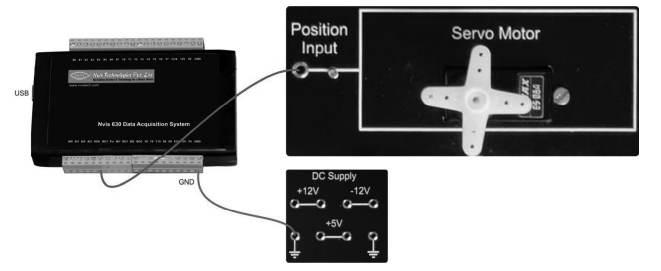
Hardware setup diagram: NVIS 630 DAQ connected via USB to the PC. The DAQ's position input terminals are wired to the servo motor position input on the NVIS 3000A kit. DC power supply (+12 V, −12 V, +5 V) provides power to the kit.
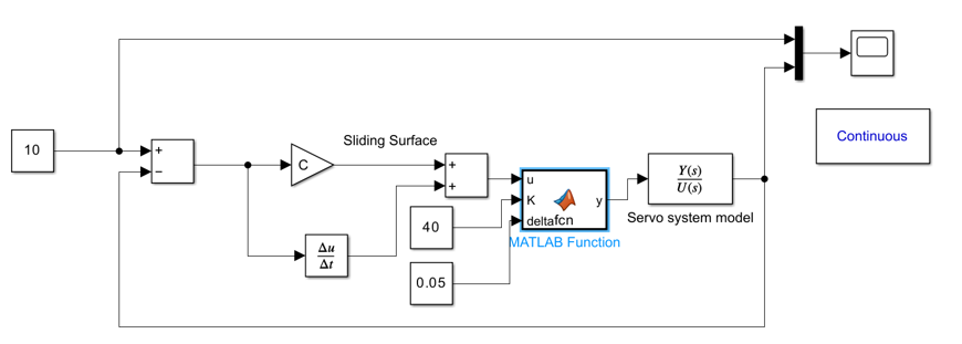
Simulink control block diagram for servo position control. A step reference input of amplitude 10 is fed to a summing junction. The error passes through a sliding surface block and a control block (gain K = 40, MATLAB Function 'deltafcn' with gain 0.05) to generate the control signal U(s). The servo system model Y(s)/U(s) produces the position output, which is fed back to close the loop. A 'Continuous' scope block records the output.
Procedure
- Connect the NVIS 630 DAQ to the PC via USB. Connect the DAQ position input terminals to the servo motor position input terminals on the NVIS 3000A kit.
- Connect the DC power supply (+12 V, −12 V, +5 V) to the NVIS 3000A kit and power it on.
- Open MATLAB/Simulink on the PC and load the servo motor position control model as shown in the Simulink diagram.
- Set the step reference input amplitude to the desired position setpoint (e.g., 10 units corresponding to the target angle).
- Configure the NVIS 3000A software on the PC to interface with the DAQ and the servo motor. Verify the COM port connection is established (indicated as 'COMS connected' in the software).
- Run the Simulink model in real-time (hardware-in-the-loop) mode. The control signal is sent to the servo motor via the DAQ, and the actual position feedback is received back.
- Observe the servo motor angle displayed in the NVIS Servo Motor Control panel. Record the initial and final positions.
- Observe the position vs time response plot in Simulink. Record the key performance parameters: rise timerise timeThe time required for a system's transient response to rise from 10% to 90% (typically for overdamped systems) or 0% to 100% (for underdamped systems) of its final steady-state value., settling timesettling timeThe time required for a system's response curve to reach and permanently stay within a specified tolerance band (usually 2% or 5%) of the final steady-state value., overshoot, and steady-state error.
- Tune the controller gains (K, sliding surface parameters) if required to improve the transient responsetransient responseThe temporary behavior of a circuit immediately after a switching event or disturbance, before it reaches its new steady-state condition..
- Switch off the power supply after completing all observations.
Simulation / Execution
Observations
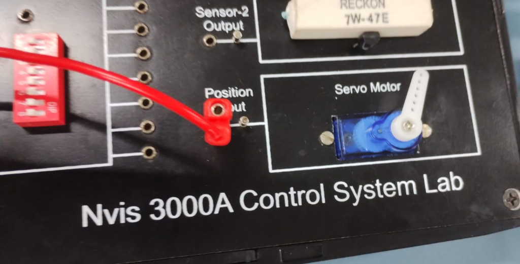
Figure 1: Physical setup showing the RECKON 7W-47E servo motor and position input terminals mounted on the NVIS 3000A panel.
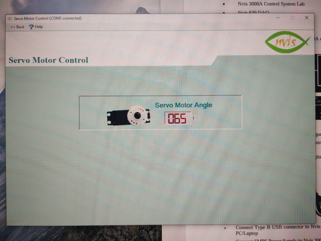
Figure 2: NVIS 3000A Servo Motor Control software display showing the real-time servo motor angle reading of 065° during position control. The COMS connection (NVIS 630 DAQ) is confirmed as connected.
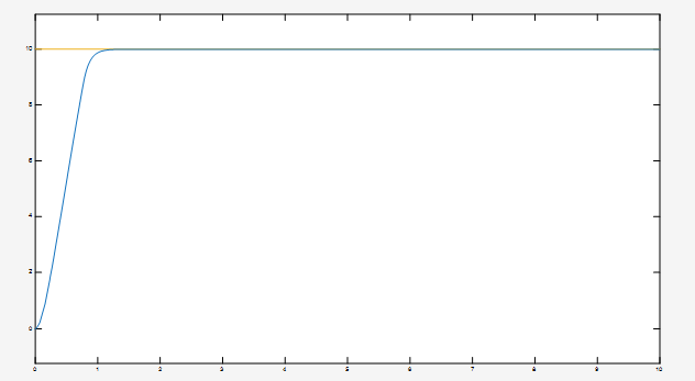
Figure 3: Servo motor position (in normalized units) vs time response from Simulink scope. The output rises rapidly from 0 to the desired setpoint of 10 units within approximately 2 seconds, showing a smooth first-order-like response with negligible overshoot and minimal steady-state error, confirming precise and stable position tracking under closed-loop control.
Calculations
| Performance Parameter | Observed Value |
|---|---|
| Rise Time (10%–90% of final value) | ≈ 1.5 s |
| Settling Time (±2% of final value) | ≈ 2.5 s |
| Maximum Overshoot | ≈ 0% (negligible) |
| Steady-State Error | ≈ 0 (negligible) |
| Final Position | 10 units (target reached) |
Results & Analysis
- The servo motor successfully tracked the desired position setpoint (10 units / 65°) with negligible steady-state error under closed-loop control, confirming accurate position regulation.
- The position vs time response showed a smooth, monotonically rising profile with negligible overshoot, indicating that the controller gains were well-tuned for this servo system.
- The rise time of approximately 1.5 s and settling time of approximately 2.5 s demonstrate fast and stable position acquisition.
- The closed-loop feedback mechanism effectively rejected the influence of any load disturbances and motor nonlinearities (friction, backlash), resulting in accurate and repeatable positioning.
- The NVIS Servo Motor Control software confirmed real-time connectivity and correct angle readout, validating the hardware-in-the-loop implementation.
- The implementation demonstrates that PID / sliding-mode-based closed-loop control provides significantly better position accuracy and stability compared to open-loop control, where position errors would accumulate without correction.
Conclusion
Post-Lab / Viva Voce
- Q: A servo motor is classified as a closed-loop control device. Explain the complete signal flow from the position reference input to the motor shaft movement, identifying each component's role in the feedback loop.
A: The signal flow is as follows: (1) Reference input — the desired position setpoint (e.g., 10 units / 65°) is specified as a step command in the MATLAB/Simulink model or via the NVIS software. (2) Error computation — the summing junction computes the error e = θref − θactual, where θactual is the position feedback from the servo's internal potentiometer/encoder. (3) Controller — the PID or sliding surface controller processes the error and produces a control signal u(t) = f(e, ė, ∫e·dt), which determines the magnitude and direction of motor drive. (4) Power amplifier / driver — the control signal is amplified to sufficient voltage and current to drive the DC motor armature. (5) DC motor + gear mechanism — the armature current produces motor torque, which is amplified by the gear train to rotate the output shaft toward the desired position. (6) Position sensor (potentiometer) — the shaft position is continuously measured and converted to a voltage proportional to the actual angle. (7) Feedback path — this feedback voltage is sent back to the summing junction, closing the loop. The motor decelerates and stops when e ≈ 0, i.e., when the actual position matches the reference. - Q: The Simulink model for this experiment uses a 'sliding surface' control block rather than a standard PID block. Explain the principle of sliding mode control (SMC) and what advantage it offers over conventional PID for servo position control.
A: Sliding mode control (SMC) is a nonlinear robust control technique that operates by driving the system state onto a predefined sliding surface s(x) = 0 in the state space and then constraining it to slide along this surface toward the equilibrium. For a servo position control system with state variables x1 = θ (position) and x2 = dθ/dt (velocity), a typical sliding surface is s = c·x1 + x2, where c > 0 determines the closed-loop dynamics on the surface. The control law has two components: an equivalent control ueq (which keeps the state on the surface once reached) and a switching control usw = K·sign(s) (which drives the state onto the surface). The key advantages over PID for servo control are: (1) Robustness — SMC is inherently robust to parameter uncertainties and external disturbances; once on the sliding surface, the dynamics are governed solely by the surface equation, not by plant parameters. (2) Finite-time convergence — the switching term drives the state to the surface in finite time, unlike PID which converges asymptotically. (3) No need for precise plant model — SMC can stabilize a system even with significant model uncertainties, whereas PID gains must be re-tuned if the plant changes. The main drawback is chattering — high-frequency switching of the control signal — which can excite mechanical resonances and wear actuators. - Q: The servo motor observed in this experiment exhibited negligible overshoot in its position response. However, a poorly tuned servo with high proportional gain exhibits significant position overshoot followed by oscillations. Explain the physical sequence of events that causes overshoot in a position-controlled servo system.
A: When a large step reference is applied, the initial position error is large, causing the PID controllerpid controllerA generic control loop feedback mechanism (Proportional-Integral-Derivative) widely used in industrial control systems to continuously calculate an error value and apply a precise dynamic correction. to apply maximum drive voltage to the motor, accelerating the shaft rapidly toward the target. As the shaft approaches the target, the position error decreases (e → 0), but the motor shaft has accumulated significant kinetic energy (angular momentum) due to the rotor inertia. The control output (which is proportional to error) reduces as the shaft nears the target, but the momentum of the rotating mass carries the shaft past the target position — this is overshoot. The position error then reverses sign (actual position exceeds reference), causing the controller to apply braking current to decelerate and reverse the motor. If the proportional gain Kp is very high, the braking effort is also large, causing the shaft to overshoot in the reverse direction. This continues as a decaying oscillation around the setpoint. The derivative term Kd reduces overshoot by sensing the angular velocity (rate of change of error) and applying pre-emptive braking before the shaft reaches the target, counteracting the momentum effect. - Q: PWM (Pulse Width Modulation) is used to control the angular position of a servo motor. Explain how the pulse width encodes the desired angle, and describe the internal mechanism by which the servo interprets this signal.
A: In a standard RC servo, position is encoded in the pulse width of a PWM signal with a fixed period of 20 ms (50 Hz). A pulse width of 1.0 ms commands full counter-clockwise position (0°), a pulse width of 1.5 ms commands the center position (90°), and a pulse width of 2.0 ms commands full clockwise position (180°). The servo's internal control circuit — typically an analog comparator or a microcontroller — decodes the pulse width by measuring its duration using a timing circuit. This duration is converted to an analog reference voltage proportional to the desired angle. The potentiometer on the output shaft generates another analog voltage proportional to the actual shaft angle. The internal error amplifier computes the difference between these two voltages (desired minus actual) and drives the DC motor in the direction that reduces this difference. The motor continues to rotate until the potentiometer voltage matches the command voltage, at which point the error is zero and the motor stops — completing the position servo loop entirely within the servo module itself. - Q: In the NVIS 3000A implementation, the position output is measured by 'Sensor-2 Output' in addition to the 'Position Output'. What is the role of having a secondary sensor output in a servo control system, and how could it be used to implement velocity feedback (tachometer feedback) to improve damping?
A: In a position control servo system, the primary feedback signal (Position Output) provides θ(t) — the shaft angle — which closes the position loop. A secondary sensor output (Sensor-2) could provide either a differentiated version of the position signal (approximating dθ/dt, angular velocity) or a direct velocity measurement from a tachogenerator if one is fitted. Velocity feedback (tachometer feedback) is an inner loop within the position control outer loop — it is a classical cascade (minor loop) control structure. The inner velocity loop, with gain Ktacho, effectively adds damping to the position loop. Analytically, for a DC motor plant G(s) = Km/(s(τs+1)), adding tachometer feedback Ktacho in a minor loop around the motor produces a modified plant G'(s) = Km/(s(τs+1+Km·Ktacho)), which has increased effective damping. This allows the outer position loop proportional gain to be increased without causing overshoot, achieving a faster, better-damped response than PID position control alone. In practice, this is implemented in the NVIS system by connecting Sensor-2 output (velocity-proportional signal) as an additional feedback input to the summing junction or as a derivative feedforward term in the controller. - Q: The closed-loop transfer function for the servo position control system is T(s) = G(s) / (1 + G(s)H(s)). If the servo plant is modeled as G(s) = Km / (s(Js+B)) (a Type 1 system, where J is rotor inertia and B is viscous friction), and H(s) = 1 (unity position feedback), show that the steady-state position error for a step input is theoretically zero, and determine the steady-state error for a ramp input.
A: The open-loop transfer function is L(s) = G(s)H(s) = Km / (s(Js+B)). The system is Type 1 (one integrator in the open-loop). For a step input R(s) = 1/s: the steady-state error is ess = lim(s→0) s·E(s) = lim(s→0) s·R(s)/(1+L(s)) = lim(s→0) s·(1/s) / (1 + Km/(s(Js+B))) = lim(s→0) 1 / (1 + Km/(s(Js+B))). As s→0, Km/(s(Js+B)) → ∞, so ess = 1/(1+∞) = 0. The position error constant Kp_pos = lim(s→0) L(s) = ∞ for a Type 1 system, confirming zero steady-state error for step inputs. For a ramp input R(s) = 1/s²: the velocity error constant is Kv = lim(s→0) s·L(s) = lim(s→0) s·Km/(s(Js+B)) = Km/B. The steady-state error for a ramp is ess_ramp = 1/Kv = B/Km. This is non-zero and inversely proportional to the motor gain constant Km — a higher motor gain or lower friction gives a smaller ramp tracking error. To achieve zero ramp tracking error, a Type 2 system (two integrators in the open loop) would be required.
References & Resources (Not Applicable)
This section is not required for this experiment.
Was this experiment helpful?
Your feedback helps us improve
Please Sign In to rate this experiment.