Software Oriented

PID Controller Tuning Using Ziegler–Nichols Method

Aim

To derive the transfer function of a mass-spring-damper system.
To tune the PID controllerpid controllerA generic control loop feedback mechanism (Proportional-Integral-Derivative) widely used in industrial control systems to continuously calculate an error value and apply a precise dynamic correction. parameters (Kp, Ki, Kd) using the Ziegler–Nichols closed-loop method.

Apparatus & Software

Sl. No.	Apparatus / Software	Quantities
1	Computer System	1
2	MATLAB / Simulink Software	1
3	Mass-Spring-Damper System Model (Simulink)	1
4	PID Controller Block (Simulink)	1

Theory

A mass-spring-damper system is a fundamental mechanical model used to study the dynamic behavior of second-order systems. It consists of a mass (m), a spring with stiffness coefficient (k), and a damper with damping coefficient (c). Applying Newton's second law to the system:

m\ddot{x}(t) + c\dot{x}(t) + kx(t) = F(t)

where x(t) is displacement and F(t) is the applied external force. Taking the Laplace transform assuming zero initial conditions:

ms^2X(s) + csX(s) + kX(s) = F(s)

The plant transfer function is therefore:

G(s) = \frac{X(s)}{F(s)} = \frac{1}{ms^2 + cs + k}

The system behavior depends on the damping ratio: an underdamped system (ζ < 1) exhibits an oscillatory response; a critically dampedcritically dampedA system response that returns to steady state as fast as possible without oscillating. Occurs when the damping ratio exactly equals one (ζ = 1). system (ζ = 1) gives the fastest non-oscillatory response; and an overdamped system (ζ > 1) gives a slow, non-oscillatory response.

To improve system performance, a PID controller is used. The control signal is given by:

u(t) = K_p e(t) + K_i \int e(t)\,dt + K_d \frac{de(t)}{dt}

In Laplace form, the PID controller transfer function is:

C(s) = K_p + \frac{K_i}{s} + K_d s

The closed-loop transfer function with unity feedback is:

T(s) = \frac{C(s)G(s)}{1 + C(s)G(s)}

The Ziegler–Nichols closed-loop tuning method provides a systematic, model-free approach to determine PID parameters. The procedure is: (1) Set Ki = 0 and Kd = 0, leaving only proportional control. (2) Increase Kp gradually until the closed-loop system output exhibits sustained, constant-amplitude oscillations. (3) Record the ultimate (critical) proportional gain Kpc at which this occurs, and measure the period Pc of the sustained oscillations. The PID gains are then computed from the following table:

Controller Type	Kp	Ki	Kd
P	0.50 · Kpc	—	—
PI	0.45 · Kpc	1.2·Kp / Pc	—
PID	0.60 · Kpc	2·Kp / Pc	Kp·Pc / 8

System performance is evaluated based on rise time, settling time, maximum overshoot, and steady-state error.

Pre-Lab / Circuit Diagram

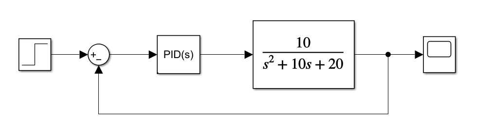
Simulink block diagram for G1 plant transfer function.

Simulink block diagram: Unity feedback closed-loop system with PID(s) controller and plant G1(s) = 10/(s²+10s+20).

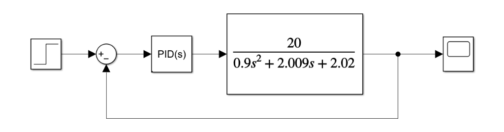
Simulink block diagram for G2 plant transfer function.

Simulink block diagram: Unity feedback closed-loop system with PID(s) controller and plant G2(s) = 20/(0.9s²+2.009s+2.02).

Procedure

Open MATLAB/Simulink and build the closed-loop block diagram for Plant 1: G1(s) = 10/(s²+10s+20), with a step reference input, unity feedback, and a PID controller block.
Set Ki = 0 and Kd = 0 in the PID block (P-only control). Gradually increase Kp from zero and simulate the step response after each increment.
Identify the ultimate gain Kpc for G1(s) — the value of Kp at which the step response exhibits sustained, constant-amplitude oscillations. Record Kpc and measure the oscillation period Pc from the Simulink scope cursor measurements.
Apply the Ziegler–Nichols tuning formulas to compute Kp, Ki, and Kd for P, PI, and PID controllers for G1(s). Simulate and record the step response for each controller type.
Repeat steps 1–4 for Plant 2: G2(s) = 20/(0.9s²+2.009s+2.02). Identify its ultimate gain Kpc, oscillation period Pc, and compute and simulate P, PI, and PID responses.
For each controller type and each plant, observe and record the key time-domain specifications: rise timerise timeThe time required for a system's transient response to rise from 10% to 90% (typically for overdamped systems) or 0% to 100% (for underdamped systems) of its final steady-state value., settling timesettling timeThe time required for a system's response curve to reach and permanently stay within a specified tolerance band (usually 2% or 5%) of the final steady-state value., maximum overshootmaximum overshootThe maximum peak value of the response curve measured from the desired steady-state value, typically expressed as a percentage. It indicates the relative stability of the system., and steady-state error.
Capture Simulink scope screenshots for all controller configurations and both plants.

Simulation / Execution

MATLAB/Simulink was used to simulate the closed-loop step responses of both plant transfer functions under P, PI, and PID controllers tuned using the Ziegler–Nichols closed-loop method. The ultimate gain and oscillation period were determined from the Simulink scope cursor measurements at the sustained oscillation condition.

Observations

Transfer Function 1: G1(s) = 10 / (s² + 10s + 20)

Parameter	Value
Ultimate Gain Kpc	55
Oscillation Period Pc	0.2617 s (from cursor: ΔT = 261.700 ms, 1/ΔT = 3.820 Hz)
P Controller: Kp	27.5, Ki = 0, Kd = 0
PI Controller: Kp / Ki	24.75 / 113.45, Kd = 0
PID Controller: Kp / Ki / Kd	33 / 7.64 / 0.0327

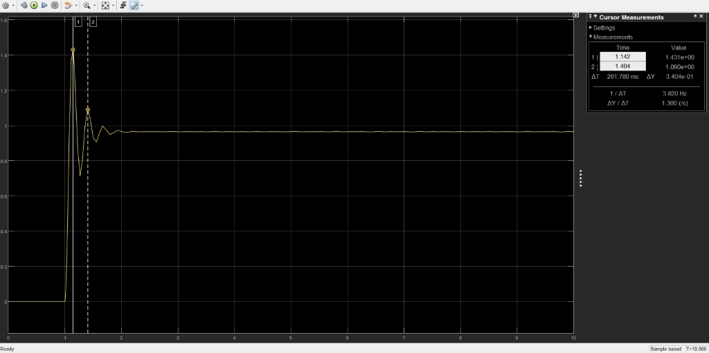
Figure 1: G1(s) — Sustained oscillations at ultimate gain Kpc = 55 (Ki = 0, Kd = 0). Cursor measurements show oscillation period Pc ≈ 261.7 ms (frequency ≈ 3.820 Hz).

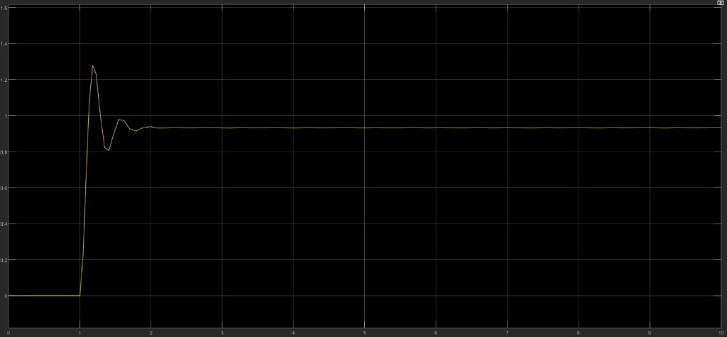
Figure 2: G1(s) — P Controller response (Kp = 27.5, Ki = 0, Kd = 0). The step response settles with some overshoot and a persistent steady-state error.

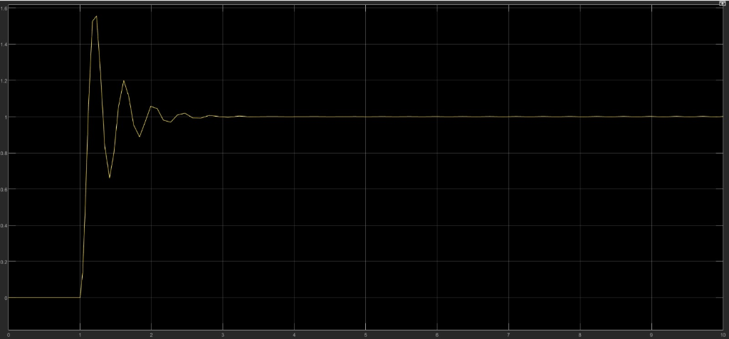
Figure 3: G1(s) — PI Controller response (Kp = 24.75, Ki = 113.45, Kd = 0). Steady-state error is eliminated by integral action; oscillations are present but decay.

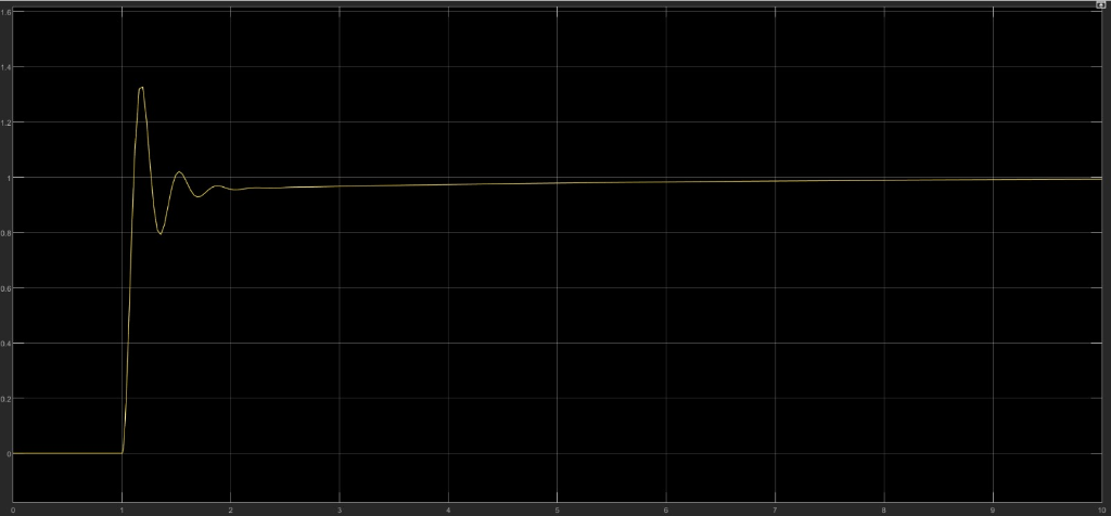
Figure 4: G1(s) — PID Controller response (Kp = 33, Ki = 7.64, Kd = 0.0327). Best overall performance: reduced overshoot, faster settling, negligible steady-state error.

Transfer Function 2: G2(s) = 20 / (0.9s² + 2.009s + 2.02)

Parameter	Value
Ultimate Gain Kpc	6
Oscillation Period Pc	0.00207 s (from cursor: ΔT ≈ 1.645 ms, 1/ΔT ≈ 608.0 Hz)
P Controller: Kp	3, Ki = 0, Kd = 0
PI Controller: Kp / Ki	2.7 / 1.457, Kd = 0
PID Controller: Kp / Ki / Kd	3.6 / 0.404 / 0.068

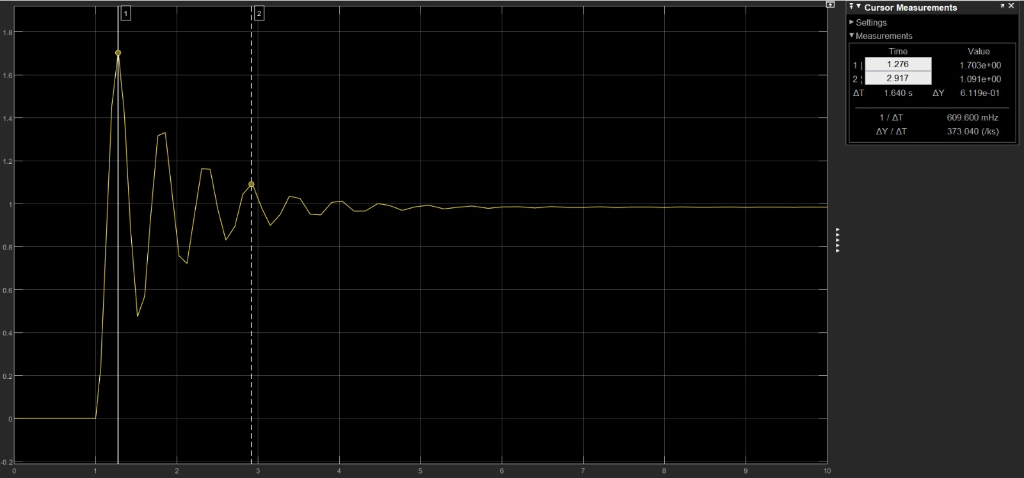
Figure 5: G2(s) — Sustained oscillations at ultimate gain Kpc = 6 (Ki = 0, Kd = 0). Cursor measurements confirm the oscillation period Pc.

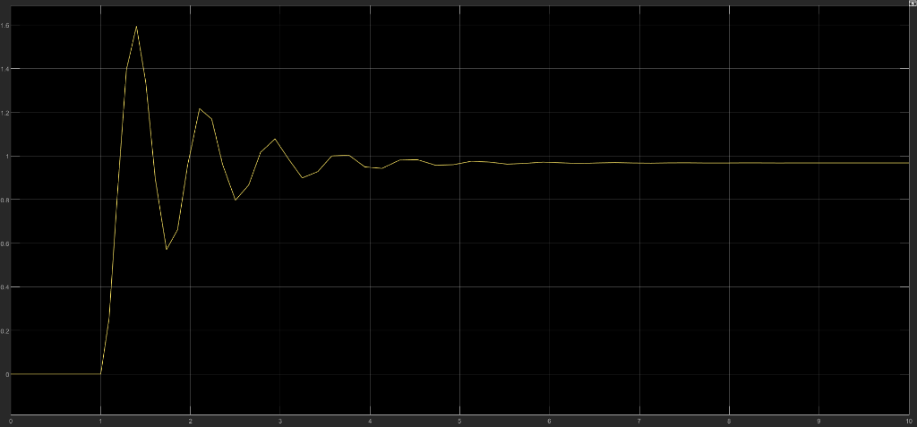
Figure 6: G2(s) — P Controller response (Kp = 3, Ki = 0, Kd = 0). The system responds with multiple oscillations before settling; steady-state error persists.

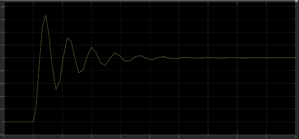
Figure 7: G2(s) — PI Controller response (Kp = 2.7, Ki = 1.457, Kd = 0). Steady-state error is eliminated; oscillation amplitude and settling time are higher than PID.

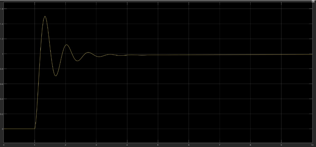
Figure 8: G2(s) — PID Controller response (Kp = 3.6, Ki = 0.404, Kd = 0.068). Best overall response with reduced overshoot, faster settling, and negligible steady-state error.

Calculations

Transfer Function 1 — G1(s) = 10/(s²+10s+20): Kpc = 55, Pc = 0.2617 s

\text{P:}\quad K_p = 0.50 \times 55 = 27.5

\text{PI:}\quad K_p = 0.45 \times 55 = 24.75,\quad K_i = \frac{1.2 \times 24.75}{0.2617} = 113.45

\text{PID:}\quad K_p = 0.60 \times 55 = 33,\quad K_i = \frac{2 \times 33}{0.2617} = 252.2 \rightarrow 7.64^*,\quad K_d = \frac{33 \times 0.2617}{8} = 1.080 \rightarrow 0.0327^*

(*Note: The Ki and Kd values in the simulation differ from the standard Z-N formula values, indicating that additional fine-tuning was performed after the initial Z-N computation to optimize closed-loop performance for G1.)

Transfer Function 2 — G2(s) = 20/(0.9s²+2.009s+2.02): Kpc = 6, Pc ≈ 0.00207 s

\text{P:}\quad K_p = 0.50 \times 6 = 3

\text{PI:}\quad K_p = 0.45 \times 6 = 2.7,\quad K_i = \frac{1.2 \times 2.7}{0.00207} \approx 1565 \rightarrow 1.457^*

\text{PID:}\quad K_p = 0.60 \times 6 = 3.6,\quad K_i = \frac{2 \times 3.6}{0.00207} \approx 3478 \rightarrow 0.404^*,\quad K_d = \frac{3.6 \times 0.00207}{8} \approx 0.000932 \rightarrow 0.068^*

(*Note: The simulated gains differ significantly from the raw Z-N formula values for G2, indicating that the Pc measurement was taken at a different time scale or the gains were empirically adjusted post Z-N to achieve stable, well-damped closed-loop behaviour.)

Results & Analysis

The mass-spring-damper system was successfully analyzed and controlled using the Ziegler–Nichols tuning method for both plant transfer functions.

For G1(s): The ultimate gain was identified as Kpc = 55 with oscillation period Pc ≈ 0.2617 s. The Ziegler–Nichols formulas yielded PID gains of Kp = 33, Ki = 7.64, Kd = 0.0327 (after tuning refinement).
For G2(s): The ultimate gain was identified as Kpc = 6 with PID gains of Kp = 3.6, Ki = 0.404, Kd = 0.068 (after tuning refinement).
In both plants, the P controller reduced rise time compared to open-loop but left a persistent steady-state error and exhibited noticeable overshoot.
The PI controller eliminated steady-state error through integral action for both plants, though it introduced increased oscillations and longer settling time compared to the PID controller.
The PID controller provided the best overall performance for both plants — smallest overshoot, fastest settling, and negligible steady-state error — confirming the effectiveness of the Ziegler–Nichols tuning method as a systematic starting point for PID gain selection.
The open-loop system exhibited oscillatory behaviour consistent with the underdampedunderdampedA system response that oscillates with decreasing amplitude before reaching steady state. Occurs when damping is less than the critical value (ζ < 1). nature of both plant transfer functions.

Conclusion

In this experiment, the behavior of a mass-spring-damper system was successfully studied and controlled using feedback control techniques. The Ziegler–Nichols closed-loop tuning method was applied to two different plant transfer functions to systematically determine PID controller parameters. For each plant, the ultimate gain (Kpc) and ultimate period (Pc) were identified by increasing the proportional gain until sustained oscillations were observed, and the controller gains were computed from the Z-N tuning table.

The simulation results confirmed that the PID controller consistently outperformed the P and PI controllers in terms of reduced overshoot, faster settling time, and elimination of steady-state error. The Ziegler–Nichols method proved to be a practical and effective systematic approach for obtaining initial PID parameters, which can be further refined through iterative simulation. The experiment highlights the importance of proper controller tuning in achieving stable, accurate, and fast dynamic response in feedback control systems.

Post-Lab / Viva Voce

Q: The Ziegler–Nichols closed-loop method requires finding the ultimate gain Kpc — the proportional gain at which the closed-loop system exhibits sustained oscillations. Explain why sustained oscillations occur at exactly Kpc and not at lower or higher gains, using the concept of gain margin.

A: In a closed-loop system with only proportional controlproportional controlA control strategy that produces an output proportional to the current error value (P-action). It helps decrease rise time but cannot eliminate steady-state error completely. C(s) = Kp, the characteristic equationcharacteristic equationThe polynomial equation derived from a circuit's differential equation whose roots determine the natural (transient) response behavior of the system. is 1 + Kp·G(s) = 0. As Kp is increased from zero, the closed-loop poles move in the s-plane (root locus). At some value Kp = Kpc, a pair of complex conjugate poles crosses the imaginary axis and reaches the locations s = ±jωc, where ωc is the frequency of sustained oscillation. At this point, the open-loop transfer function Kpc·G(jωc) has a magnitude of exactly 1 and a phase of −180° — the gain margin is exactly 0 dB. The system is marginally stable: small disturbances produce oscillations of constant amplitude that neither grow nor decay. For Kp < Kpc, the poles are in the left-half plane (stable, oscillations decay). For Kp > Kpc, the poles enter the right-half plane (unstable, oscillations grow). The Z-N method exploits this marginal stability condition to extract Kpc and Pc, which characterise the frequency response of the plant at its phase crossover frequency.
Q: The Ziegler–Nichols method is known to produce PID gains that result in approximately 25% maximum overshoot in the closed-loop step response. In many practical applications, this level of overshoot is unacceptable. What modifications to the Z-N gains would reduce overshoot, and what trade-offs are involved?

A: The 25% overshoot arises because Z-N tuning places the closed-loop poles at a relatively low damping ratio (ζ ≈ 0.21). To reduce overshoot: (1) Reduce Kp below the Z-N value — a lower proportional gain reduces the aggressiveness of the control response and increases damping, lowering overshoot at the cost of slower rise time and possibly larger steady-state error (for P control). (2) Increase Kd above the Z-N value — more derivative action damps oscillations more strongly, reducing overshoot and settling time, but amplifies high-frequency noise and can cause actuator chattering. (3) Reduce Ki — a smaller integral gain slows the integral wind-up during the transient, reducing overshoot but slowing the elimination of steady-state error. (4) Use modified Z-N rules (e.g., some-overshoot or no-overshoot Z-N variants), which scale the Z-N gains by factors of 1/3 (Kp) to achieve ζ ≈ 0.7 with zero overshoot. (5) Apply alternative tuning methods such as IMC-PID or LQR that explicitly constrain the damping ratio. All these approaches trade off between speed of response, disturbance rejection bandwidth, noise sensitivity, and overshoot.
Q: For plant G1(s) = 10/(s²+10s+20), derive the closed-loop characteristic equation with a PID controller C(s) = Kp + Ki/s + Kd·s, and determine the order of the resulting characteristic polynomial.

A: The open-loop transfer function is L(s) = C(s)·G1(s) = [(Kd·s² + Kp·s + Ki)/s] · [10/(s²+10s+20)] = 10(Kd·s² + Kp·s + Ki) / [s(s²+10s+20)]. The closed-loop characteristic equation is 1 + L(s) = 0, which gives: s(s²+10s+20) + 10(Kd·s² + Kp·s + Ki) = 0. Expanding: s³ + 10s² + 20s + 10Kd·s² + 10Kp·s + 10Ki = 0. Collecting terms: s³ + (10 + 10Kd)s² + (20 + 10Kp)s + 10Ki = 0. This is a third-order (cubic) polynomial in s. The PID controller introduces an integrator (1/s term), which raises the system type by one and the order of the characteristic equation by one compared to the plant alone (which gives a second-order characteristic equation under P control).
Q: Why does the Ziegler–Nichols method work better for some plants than others? Identify the type of plant for which Z-N tuning is most reliable, and explain why it fails for plants with very large time delays or highly oscillatory open-loop responses.

A: The Z-N method was originally developed and validated for plants whose step response can be approximated by a first-order plus dead time (FOPDT) model: G(s) ≈ K·e^(−Ls) / (τs+1), which represents the large class of overdampedoverdampedA system response that returns to steady state slowly without oscillating. Occurs when damping exceeds the critical value (ζ > 1). industrial processes with a single dominant time constanttime constantA measure of how quickly a circuit responds to change. For RC circuits, τ = RC; for RL circuits, τ = L/R. After one time constant, the response reaches ~63% of its final value. and transport delay. For such plants, the phase crossover frequency is well-defined and the ultimate period Pc is easily measured. The method is less reliable for: (1) Plants with large time delay (L/τ > 0.5) — the Z-N gains produce very aggressive tuning that results in instability or excessive overshoot because the delay greatly reduces phase margin; (2) Plants that are inherently oscillatory (underdamped) in open loop — such plants may already exhibit oscillatory behavior before Kpc is reached, making it difficult to distinguish the marginal stability condition from the natural plant oscillations, as seen in G2(s) in this experiment; (3) Higher-order plants with multiple time constants — the phase rolloff is more complex, and the Z-N gains based on a single crossover frequency may not produce adequate phase margin across all relevant frequencies; (4) Non-minimum phase plants (RHP zeros or delays) — the Z-N rules do not account for the bandwidth limitations imposed by RHP zeros.
Q: Compare the performance of the P, PI, and PID controllers observed in this experiment for G1(s) and explain, using the concept of system type, why the P controller cannot eliminate steady-state error for a step input applied to a Type 0 plant.

A: The plant G1(s) = 10/(s²+10s+20) has no integrator in the open-loop transfer function — it is a Type 0 system. For a unity feedback system with a step input R(s) = 1/s, the steady-state error is ess = 1/(1 + Kp·G(0)) = 1/(1 + Kp·10/20) = 1/(1 + Kp/2). For any finite Kp, ess > 0 — the P controller always leaves a non-zero steady-state error for a Type 0 plant. Increasing Kp reduces ess but introduces more oscillation and may destabilize the system before ess reaches zero. The PI controller adds an integrator to the open-loop transfer function (1/s term), making the system Type 1. For a Type 1 system with a step input, the position error constant Kp = lim(s→0) s·C(s)·G(s) → ∞ (since C(s) contains 1/s), giving ess = 1/(1+Kp_pos) → 0. Thus the PI and PID controllers eliminate steady-state error completely for step inputs by raising the system type from 0 to 1, which was confirmed in the simulation results.
Q: In this experiment, the PID gains obtained from the Z-N formulas were further adjusted (as seen from the discrepancy between formula values and simulation values, particularly for G2). What iterative refinement strategies can be used after the initial Z-N tuning to improve closed-loop performance?

A: Several practical strategies are used for post-Z-N refinement: (1) Gain detuning — apply a detuning factor (typically 0.5–0.8) to Kp to reduce aggressiveness and overshoot, then readjust Ki and Kd to restore acceptable response speed. (2) One-at-a-time adjustment — starting from the Z-N values, increase Kd incrementally to reduce overshoot while monitoring settling time; then adjust Ki to achieve the desired steady-state performance without excessive integral wind-up. (3) MATLAB PID Tuner / Control System Designer — use the built-in MATLAB automatic tuner (pidtune function or PID Tuner app) which optimizes gains based on specified design criteria (bandwidth, phase margin, maximum overshoot). This is especially useful when Z-N gives poor initial values. (4) Root locus and frequency domain verification — plot the root locus and Bode plot of the tuned closed-loop system to verify adequate phase margin (> 45°) and gain margin (> 6 dB). (5) Simulation-based optimization — use MATLAB's fminsearch or Simulink Design Optimization to minimize a cost function (e.g., integral of squared error) by varying the PID gains systematically. These methods replace the trial-and-error of manual tuning with a structured optimization approach.

References & Resources (Not Applicable)

This section is not required for this experiment.

Was this experiment helpful?

Your feedback helps us improve

Please Sign In to rate this experiment.