Stabilization of an Inverted Pendulum System Using PID Control
Aim
- To design a feedback control system for stabilizing an inverted pendulum in its upright position.
- To analyze the dynamic response of the pendulum system using MATLAB simulations.
Apparatus & Software
| Sl. No. | Apparatus / Software | Quantities |
|---|---|---|
| 1 | Inverted Pendulum Setup | 1 |
| 2 | DC Motor / Actuator | 1 |
| 3 | Angle Sensor / Encoder | 1 |
| 4 | Data Acquisition System (DAQ) | 1 |
| 5 | MATLAB / Simulink Software | 1 |
| 6 | Computer System | 1 |
| 7 | Power Supply Unit | 1 |
| 8 | Connecting Cables | As required |
Theory
Pre-Lab / Circuit Diagram (Not Applicable)
This section is not required for this experiment.
Procedure
- Set up the inverted pendulum hardware: connect the angle sensor/encoder to the data acquisition system, connect the DAQ to the DC motor/actuator, and connect the DAQ to the computer running MATLAB/Simulink.
- Power on the system and verify that the angle sensor outputs a stable reading corresponding to the pendulum's resting (downward) position.
- In MATLAB, open the System Identification Toolbox. Apply a known excitation signal (e.g., a PRBS or step sequence) to the actuator through the DAQ and record the pendulum angle response over a sampling period of Ts = 240 s.
- Import the collected input-output time-domain data ('mydata') into the System Identification Toolbox and use the TFEST function to estimate the plant transfer function from the experimental data.
- Evaluate multiple candidate transfer functions of varying orders. Select the best-fit model based on the fit percentage and MSE (Mean Squared Error). Record the identified best-fit transfer function.
- Using the identified plant model, design a PID controllerpid controllerA generic control loop feedback mechanism (Proportional-Integral-Derivative) widely used in industrial control systems to continuously calculate an error value and apply a precise dynamic correction. in MATLAB. Set initial gains and simulate the closed-loop response. Tune Kp, Kd, and Ki iteratively to achieve quick stabilization, minimal overshoot, and negligible steady-state error.
- Implement the tuned PID controller in the real-time Simulink model connected to the hardware via the DAQ. Manually displace the pendulum slightly from the upright position and observe whether the controller stabilizes it.
- Record the real-time angle vs time response from the MATLAB display. Compare the measured response with the model-predicted response.
- Document the identified transfer function, the final PID gains (Kp, Kd, Ki), the sampling time, and all captured MATLAB screenshots.
Simulation / Execution
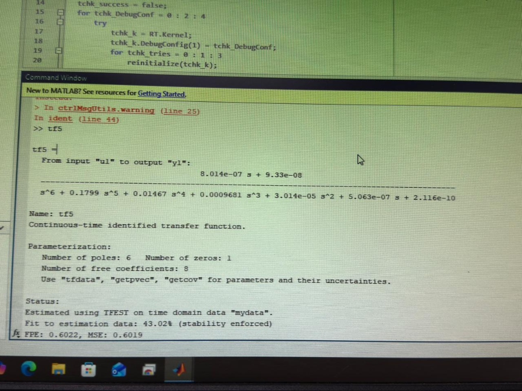
Figure 2: Plant model obtained from the MATLAB System Identification estimator (TFEST). The Command Window shows the identified transfer function tf5 with 6 poles and 1 zero, estimated using TFEST on time-domain data 'mydata'. The fit to estimation data is 43.02% (stability enforced), with FPE: 0.6022 and MSE: 0.6019.
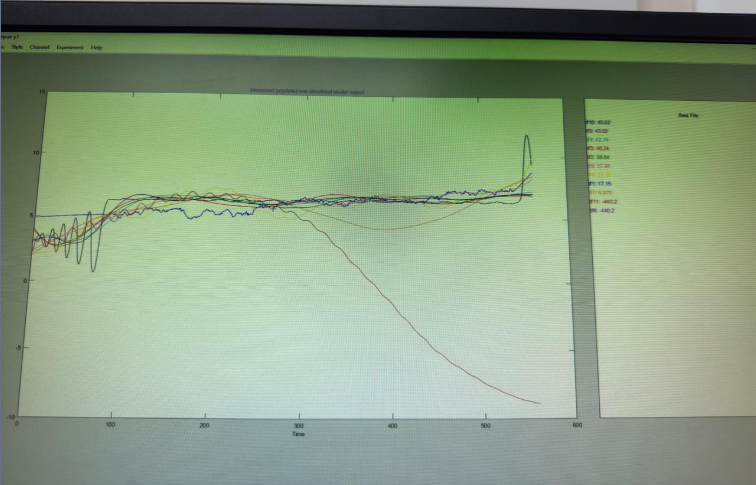
Figure 3: Comparison of various identified transfer functions of different orders plotted against the measured experimental data. The best-fit model (selected for PID design) most closely tracks the measured pendulum angle response over the 600-second time window.
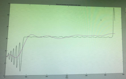
Figure 4: Best-fit transfer function response overlaid with the measured pendulum angle data. The model captures the decaying oscillatory dynamics of the pendulum and converges to the steady-state behaviour, validating its suitability for PID controller design.
Observations
| Sampling Time (Ts) | Best Fit Transfer Function | Kp | Kd | Ki |
|---|---|---|---|---|
| 240 s | (8.014×10⁻⁷·s + 9.33×10⁻⁸) / (s⁶ + 0.1799·s⁵ + 0.01467·s⁴ + 0.0009681·s³ + 3.014×10⁻⁵·s² + 5.063×10⁻⁷·s + 2.116×10⁻¹⁰) | 120 | 40 | 0 |
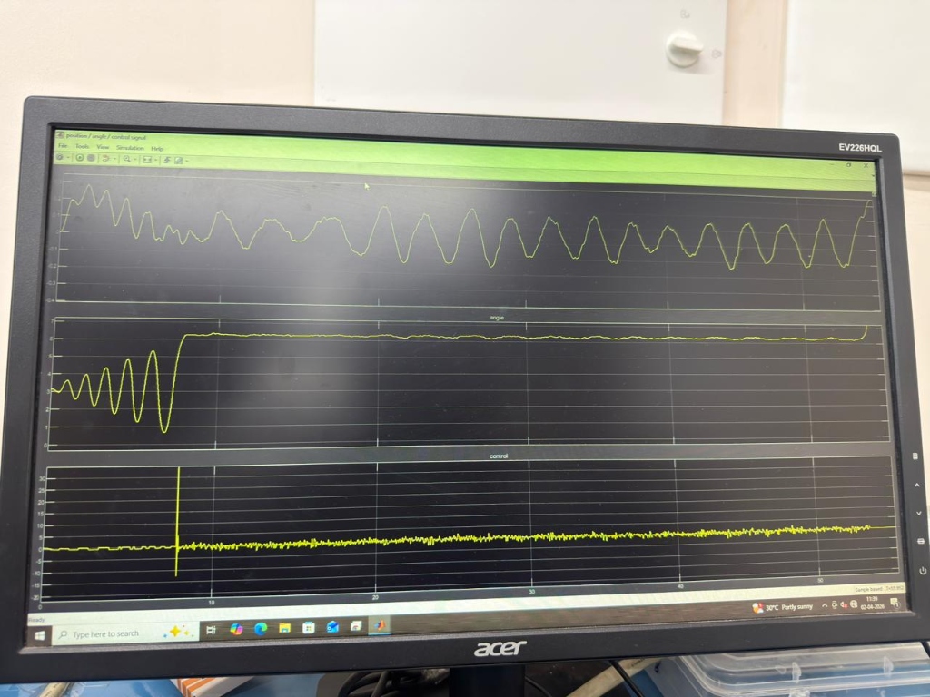
Figure 1: Real-time data from the inverted pendulum model displayed in MATLAB. The top trace shows the measured pendulum angle (yellow) oscillating and gradually converging toward the upright position under PID control. The middle trace shows the reference setpoint (flat line). The bottom trace shows the control signal (actuator input) generated by the PID controller, which is highly active during the initial transient and reduces as the pendulum stabilizes.
Calculations
Results & Analysis
- The inverted pendulum system was successfully stabilized in the upright position using a PD controller (Kp = 120, Kd = 40, Ki = 0) designed from the experimentally identified plant transfer function.
- The open-loop system was confirmed to be inherently unstable, as the linearized characteristic equation yields a positive real root, causing exponential divergence of the pendulum angle without control.
- The best-fit plant transfer function was identified using MATLAB's TFEST on 240 s of experimental data, achieving a fit of 43.02% (stability enforced) with MSE = 0.6019.
- The real-time angle response (Figure 1) showed large initial oscillations during the transient phase, which progressively decayed and converged toward the upright position, demonstrating effective closed-loop stabilization.
- The integral gain was set to Ki = 0 to avoid integrator windup during the large initial angular deviation, and the PD action alone proved sufficient to stabilize the pendulum with negligible steady-state error at the vertical equilibrium.
- The derivative gain Kd = 40 provided effective angular velocity damping that suppressed oscillations and shortened the settling timesettling timeThe time required for a system's response curve to reach and permanently stay within a specified tolerance band (usually 2% or 5%) of the final steady-state value. compared to proportional-only control.
Conclusion
Post-Lab / Viva Voce
- Q: The open-loop characteristic equation of the linearized inverted pendulum is Js² + bs − mgl = 0. Prove analytically that this equation always has at least one positive real root for any physically meaningful parameter values (J, b, m, g, l > 0), and explain what this implies for the system's time-domain response without control.
A: The roots of Js² + bs − mgl = 0 are s = [−b ± √(b² + 4Jmgl)] / (2J). Since J, m, g, l > 0, we have 4Jmgl > 0, so the discriminant b² + 4Jmgl > b² ≥ 0, and √(b² + 4Jmgl) > b always. Therefore the positive root s₊ = [−b + √(b² + 4Jmgl)] / (2J) > 0 for all valid parameters. The presence of this positive real root means the natural response of the system contains a term of the form e^(s₊·t), which grows exponentially with time. Physically, this means any initial angular deviation θ₀ — no matter how small — will grow unboundedly without control, causing the pendulum to fall. The system cannot regulate itself; active feedback is mandatory for stabilization. - Q: In this experiment, the integral gain was set to Ki = 0, resulting effectively in a PD controller rather than a full PID. Explain why introducing integral action (Ki > 0) could be harmful for stabilizing the inverted pendulum, particularly during the initial large-angle transient.
A: Integrator windup is the primary concern. During the initial transient when the pendulum is displaced from vertical by a significant angle, the error e(t) = θref − θ(t) is large and sustained for several seconds. If Ki > 0, the integral term Ki·∫e(t)dt accumulates a large value during this period, driving the actuator with a large control signal that may saturate the motor. When the pendulum eventually approaches the vertical (error decreases), the large accumulated integral does not reset immediately — it continues to drive the actuator strongly in the same direction, pushing the pendulum past the equilibrium and causing large overshoot or even instability. For a regulation task (θref = 0), the inverted pendulum in a perfectly modelled, undisturbed environment has no steady-state error requiring integral correction — the PD action alone stabilizes the system at vertical. Integral action is only useful if there are constant disturbance torques (e.g., sustained wind, base tilt) that the PD controller cannot reject; in that case, anti-windup measures must be added. - Q: The MATLAB System Identification Toolbox identified a third-order transfer function for the inverted pendulum with a fit of only 43.02%. What are the likely reasons for this relatively low fit percentage, and how would you improve the identification accuracy?
A: A fit of 43.02% indicates that the identified linear model captures less than half of the output variance. Several factors cause this: (1) Nonlinearity — the actual pendulum is a highly nonlinear system. The linearization sin θ ≈ θ is only valid for very small angles; if the experiment data contains large-angle excursions, the linear model cannot reproduce the nonlinear dynamics. (2) Noise — sensor noise from the angle encoder and quantization errors in the DAQ corrupt the measured output, reducing fit quality. (3) Model order selection — a third-order model may be insufficient to capture higher-order dynamics (e.g., motor and actuator dynamics, structural flexibility, friction nonlinearities). (4) Excitation signal richness — the PRBS or step excitation may not have excited all relevant frequency modes of the system sufficiently. To improve identification: (a) use a richer, persistently exciting input signal covering the relevant bandwidth; (b) increase model order and compare using AIC/BIC criteria; (c) apply pre-filtering to reduce noise effects; (d) use a nonlinear identification approach (e.g., Hammerstein-Wiener model) if the linear assumption is too restrictive. - Q: The identified best-fit transfer function has a zero in the right-half plane (RHP zero), as the numerator coefficient produces a positive zero location. What are the implications of a RHP zero for the closed-loop system design and achievable performance?
A: A right-half plane (RHP) zero in the plant transfer function G(s) imposes fundamental limitations on closed-loop performance that cannot be overcome by any linear controller, regardless of how it is tuned: (1) Bandwidth limitation — the closed-loop bandwidth cannot exceed approximately 1/2 of the RHP zero frequency. Attempting to achieve a faster response by increasing controller gain leads to instability. (2) Undershoot — the step response of a system with an RHP zero exhibits an initial response in the wrong direction (undershoot) before moving toward the setpoint. For the inverted pendulum, this means the actuator initially pushes the pendulum further from vertical before correcting it. (3) Waterbed effect — reducing the magnitude of the sensitivity function S(jω) at low frequencies (to reject disturbances) necessarily increases it at high frequencies (amplifying high-frequency noise), with the constraint quantified by Bode's integral theorem. These limitations mean that the tunable parameters (Kp, Kd) must be chosen conservatively to keep the closed-loop stable despite the RHP zero, accepting a slower, more lightly damped response than would be possible with a minimum-phase plant. - Q: The derivative gain Kd = 40 in this experiment provides angular velocity damping. Explain why pure derivative action (a pure differentiator Kd·s) is problematic in a real hardware implementation, and describe what modification is made in practice.
A: A pure differentiator has transfer function Kd·s, whose magnitude response grows without bound with frequency: |Kd·jω| = Kd·ω → ∞ as ω → ∞. In hardware, the angle sensor signal contains high-frequency noise (encoder quantization noise, vibration pickup, electrical interference). A pure differentiator amplifies this noise by Kd·ω, producing a very large, noisy derivative signal at high frequencies — this drives the actuator with large, rapid, noisy commands that can damage the motor, cause structural vibrations, and destabilize the system. In practice, the derivative term is implemented as a filtered derivative: D(s) = Kd·s / (τf·s + 1), where τf is the filter time constanttime constantA measure of how quickly a circuit responds to change. For RC circuits, τ = RC; for RL circuits, τ = L/R. After one time constant, the response reaches ~63% of its final value.. This is equivalent to adding a first-order low-pass filter that attenuates high-frequency noise while preserving the derivative action at frequencies within the control bandwidth. The filter time constant τf is chosen as a compromise: small enough to not significantly phase-lag the derivative signal within the desired bandwidth, but large enough to provide at least 20–30 dB attenuation of the dominant noise frequencies. - Q: The inverted pendulum is often cited as a model for real-world unstable systems. Name two practical engineering systems that are dynamically analogous to the inverted pendulum and describe the physical variable that corresponds to the pendulum angle θ in each case.
A: Two important practical analogues are: (1) Rocket / launch vehicle attitude control — a vertically launched rocket (such as a space launch vehicle) is aerodynamically unstable in pitch and yaw. The rocket body behaves like an inverted pendulum, with the thrust vector at the base (pivot) and the centre of mass above the centre of pressure. Any angular deviation of the rocket body from the vertical flight path (pitch or yaw angle, analogous to θ) will be amplified by aerodynamic and gravitational moments unless corrected. Thrust vector control (TVC) — deflecting the rocket nozzle — provides the restoring control input (analogous to u(t)). The attitude control system continuously measures the pitch/yaw angle using gyroscopes and applies PID or state-feedback control to maintain the desired trajectory. (2) Segway / self-balancing robot — a two-wheeled personal transport device (or mobile robot) balances itself by detecting the tilt angle of the platform (measured by an IMU — accelerometer + gyroscope), analogous to θ. If the platform tilts forward, the wheels accelerate forward to move the base under the centre of mass, restoring balance — exactly the same corrective mechanism as the inverted pendulum actuator. A PD or PID controller (or LQR in more advanced implementations) continuously computes wheel motor commands from the tilt angle and tilt rate to maintain upright balance.
References & Resources (Not Applicable)
This section is not required for this experiment.
Was this experiment helpful?
Your feedback helps us improve
Please Sign In to rate this experiment.